[RL]Soft-RL: Maximum Entropy Reinforcement Learning as Probabilistic Inference

The first book you read about Reinforcement Learning is likely the book Reinforcement Learning: An Introduction. In the book, dear Richard Sutton and Andrew Barto introduced reinforcement learning from the view of maximizing total Reward in very detail. The book explained reinforcement learning step by step:

1. Multi-armed Bandits problems
2. How to build a Markov Decision Process(MDPs).
3. Using Dynamic Programming to solve the MDPs.
4. Using Monte-Carlo methods to avoid computing the state dynamic transition model.
5. Using Important Sampling to keep track of behavior and target policies.
6. Temporal Difference

One of the key ideas behind this book is how to update state-action evaluation Q(s, a) and state evaluation V(s).

However, if we are modeling decision problems in Markov Decision Process, wouldn’t it be nice if we have everything in probability view? Moreover, using the probabilistic view can provide a way to model policy’s entropy. In other words, handling the exploration problem becomes more convenient. One extra problem, What is really a reward is defined as. The paper Reinforcement learning and control as probabilistic inference: Tutorial and review(1805.00909.pdf (arxiv.org)) written by Sergey Levine provided a different view.

To summarize, there are two advantages of using soft reinforcement learning:

1. Dealt with Exploration problem by limiting the entropy of policy.
2. Define how a reward function should be like.

Part 1 Models.

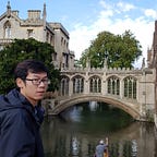
The goal of reinforcement learning is finding the optimal decisions to achieve certain goal. It requires each action selected at each step to be global optimal. For each state-action, such optimality is indicated by a probability “O” in the Probabilistic graphical model (PGMs) as (b) below. This probability is the probability of this state-action is the optimal choice. In other words, how good is this action at given state.

(a): State Transition Graph: P(s’|s, a) (b). State transition and rewards. P(s’|s, a) and P(O|s, a)

And this optimality is directly connected with how to define rewards. Same as Sutton’s book, the goal is find a parametrized policy P(a|s,θ) that maximize the overall total rewards.

The definition of a reward for each state-action should be corresponding to how close it is to the optimal action.

In order to find a way to find the optimal solution, or we say optimize the policy’s parameters to find the optimal solution, the transactions between the agent and environment is form as a trajectory. And the probability of forming such trajectory is shown as:

A trajectory is the product of “initial state probability P(s_1)” and “policy P(a_t|s_t,θ)” and “state transition probability p(s_{t+1}|s_t,a_t)”

Ant Direction Example InfoRL: Interpretable Reinforcement Learning using Information Maximization

Clearly, only having the trajectory is not enough. We need to connect rewards, or Optimality(O) here, to the trajectory.

In order to connect the optimality variable with trajectory, they defined the relationship between optimality variables and a trajectory by conditioning the trajectory on the Optimality variables. Although we assume the trajectory and optimality variables are independent(if P(τ|O) is equals 0) for now, this relationship is not wrong.

Based on the Bayes Equation, P(τ|O) = P(τ,O)* 1/P(O) where P(O) is a constant prior, then we can introduce the optimality in trajectory. And our goal now is maximizing this optimality.

As we can see, an very familiar term “Returns” become part of this equation. Actually, in a deterministic environment, where the state transition probability is 1. The rewards goal can be reduced to standard planning or trajectory optimization like what we saw in Sutton’s book.

Part 2 Modelled by Message Passing (Dynamic Programming).

It caused me a little bit confusion about Message Passing at the beginning. However, when I look into it, it is honestly just passing Q and V values.

For the future (i.e. time steps t:T), they defined the probability of having a set of optimal states as:

And they defined the probability of having optimal state-action pair in the future as:

If you are familiar with what is Q and V vales are, you may have a hint about what is these two probability linked with. But be aware that now it is just probabilities.

Remember there is a conversion between Q and V values in Sutton’s book.

Now, does it still stands? Of course it is. The Q and V depends on each other, so does the messages β(s, a) and β(s). Firstly, let’s find a way to convert Q to V. Here, we must assume that s_t and a_t are independent, so P(s_t, a_t) = p(s_t)p(a_t).

It is equivalent to V = G(Q) like the upper right Equation.

One thing worth to note is that, P(a_t|s_t) is not policy at all. It is just a constant prior. Secondly, let’s find a way to convert V to Q.

And it is proofed by:

Introduce Policy:

Firstly, based on the Markov Property, the overall optimal policy P(a_t|s_t, O_{1:T}) is not depends on the past(O_{1:t-1}), but only depends on the future(O(t:T)). Therefore, P(a_t|s_t, O_{1:T})=P(a_t|s_t, O_{t:T}).

We can easily find the optimal policy who is proportional to the β(s, a) divided by the β(s). Using bayes’ rule in the third step.

As you can notice, the way of defining and updating the β(s, a) and the β(s) are quiet similar to how we update Q and V values in standard reinforcement learning. Here we consider the β(s, a) and the β(s) as probability. They should be bounded to [0,1]. However, our Q value and V values can be any number. Let’s take a compromise, and transfer β(s, a) and the β(s) into log-space, where the Q and V values are negative.

In standard reinforcement learning, the policy is correlated with advantage function. In other words, how to choose the action is depending on the Q(s_t,a_t)-V(s_t).

And the policy is:

And the conversion between Q and V still stands.

Therefore the message passing backup in deterministic environment is :

Be aware that the above equations are assuming deterministic state transitions.

Part 3 Define Inferencing Objective(KL Divergence)

Let’s find the original definition of a trajectory with a policy making decisions.

A trajectory is the product of “initial state probability P(s_1)” and “policy P(a_t|s_t,θ)” and “state transition probability p(s_{t+1}|s_t,a_t)”

When the environment is deterministic,

And then, Let’s recall the overall distribution with the optimality variables of the trajectory graph.

And when the dynamic is deterministic, it can be simplified as:

Now the thing should become clear. The policy is updated to find the optimal solution who is as close as possible to the Equation 4. We want this KL-Divergence to be as small as possible.

Minimizing such KL-Divergence can be re-written as maximizing the negative KL-Divergence:

Vola! That’s looks very very familiar if you have ever read the paper[Soft actor-critic: Off-policy maximum entropy deep reinforcement learning with a stochastic actor]. haarnoja18b.pdf (mlr.press) It is the soft goal of reinforcement learning taking consideration of policy entropy.

Stochastic(I am not sure about this part, so I will just paste the original text, some one could enlighten me about it?):

The Soft-Bellman Updates for stochastic environment may introduce “Risk Seeking” behaviors. It is due to the soft-max operation in the last component in Equation 7 below. It will emphasize high-values and suppress low-values, even when high-value is unlikely to happen.

For stochastic environment, where the state transition probability is not 1. The dynamic and initial state term does not cancel. We use the trajectory level of KL-Divergence:

Where:

Part 4 Variational Inference and Stochastic Dynamics.

Under stochastic dynamic assumption, the goal is still maximizing the negative KL-Divergence.

However, now we are optimizing something similar to the standard reinforcement learning. Therefore, we need to find the backward messages like what we did in standard reinforcement learning. And then optimize the objective by dynamic programming.

The V(S_T) is defined as:

Which is coherent with previous definitions of :

Therefore, we want to maximize the right hand side of Equation 12.

Then the above equation 12 in the paper can be proofed by:

It is a important equation which has also been used in the paper about Soft-Actor-Critic. However, in that paper, the proof is not given clearly.

Apparently, In the KL-Divergence, when the

The KL-Divergence becomes 0 and it is the minimal. Therefore, the optimal policy is for the KL-Divergence only:

However, the V(S_T) term in Equation12 is not dealt with! We can just add one extra term to maximize both.

And the objective is rewritten as:

Here, these two assumption is hold.

Variational Inference

There is some intractable p(\tau):

We want to use some tractable approximator to approximate the intractable.

Here, if the q(s1) is defined to be equal to p(s1), and the state transition dynamics and approximated dynamics q(s_t+1|s_t,a_t) is defined to be equal as well.

Then the q(\tau) here is exactly the \hat{p(\tau)}:

Therefore, maximizing the variational lower bound in variational inferencing is trying to maximize the trajectory’s optimality log p(O_{1:T}), and this inequation is derived from Jensen’s inequality:

Jensen’s Inequality:

For more detail, A recommended paper is:

Elbo surgery: yet another way to carve up the variational evidence lower bound

If we replace the p(O_{1:T, s_{1:T}, a_{1:T}}) with the definition of rewards. and q(a_t|s_t). Then optimizing the bound is equivalent to optimizing the soft objective equation we defined before.

In the end of this paper, the author provided three soft algorithms, namely, Soft-Q learning, Soft-Actor-Critic, and Soft(Maximum Entropy) Policy Gradient. They are corresponding to the Value-based, Actor-Critic, and Policy Gradient in standard Reinforcement Learning.

Part 5 Summary

I think the prior contribution of this paper is providing a different view of reinforcement learning. The author model the solutions of Markov Decision Process as Probability Inferencing. It bring several advantages:

1. How to do exploration. The exploration here is depending on the rewards, which the policy is softly trained to approach.
2. How to define rewards. The rewards here is defined as the optimality. It is a negative number that can be converted to probability by exponential function.
3. Taking advantage of probability research which is considered to be more diverse and mature.

In this paper, there are three ways to do the optimization:

1. Message Passing: Just like what we did in standard reinforcement leanring.
2. Utilizing the KL-Divergence between optimal trajectories(where there are rewards) and policy trajectories(where there are parameterized policy).
3. Variational Lower Bound.

Although this paper has been published in 2018, and only cited around 260 times for now. I still consider this paper is a very good review for probabilistic inferencing as reinforcement learning.